Exponential Attenuation
Having reviewed how individual photons interact with matter in the photon interactions tutorial, we will now consider the macroscopic properties of a photon beam, i.e. a large collection of photons, and their composite interaction with matter. A derivation of the exponential attenuation equation will be given, followed by a discussion of the terms and conditions required to acheive the derived equation.
Derivation
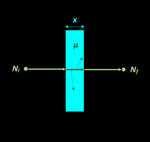
Suppose we can form an experiment involving a beam of radiation initially containing N_0 photons. This beam originates from a point source and travels in a thin, straight line. The beam travels through a vaccum (without interacting) until reaching an attenuating material with length x. While traveling through the material, some of the individual photons in the beam will undergo interactions as described in the photon interactions tutorial, but other photons will pass through the material unaffected and can be counted by a point detector in a vacuum on the other side. The figure below depicts our contrived experiment. The question we want to answer is this: what number of photons N will pass through the material unaffected, or unattenuated, and reach the detector?
We start our derivation by defining an attenuation coefficient \mu, which is the probability that a single photon will interact with the medium per unit length (usually cm or m). The units for the attenuation coefficient are usually cm-1 or m-1. Given this definition of the attenuation coefficient, the rate of change in the number of unattenuated particles dn over a length of attenuating material dl is simply equal to the interaction probablilty per particle per length (i.e. the attenuation coefficient), multiplied by the number of particles n and the material length:
dn = \mu n dl
dn = \mu n dl
dn/n = \mu dl
Integrating each side of the equation over the appropriate bounds and simplifying:
\int_{N_0}^{N}{dn/n} = \int_{0}^{x}{\mu dl}
-ln(n) \Big|_{N_0}^{N} = \mu l \Big|_{0}^{x}
-ln(N) + ln(N_0) = \mu x
ln(N) - ln(N_0) = -\mu x
ln(N/N_0) = -\mu x
N/N_0 = e^{-\mu x}
N = N_0 e^{-\mu x}
The number of unattenuated photons decreases exponentially as the material length increases, hence the name exponential attenuation.
The Attenuation Coefficient
The derived exponential attenuation was made fairly simple by our definition of the attenuation coefficient. However, since we know the probabilities of individual photon interactions as defined by their cross sections, we can calculate the attenuation coefficient as the sum of all individual interaction probabilities, using the "or rule" for probabilities:
\mu = \sigma_{R} + \sigma_{pe} + \sigma_{C} + \sigma_{pp} + \sigma_{pn}
In other words, the photon attenuation coefficient is the probability that the photon will undergo any one of these interactions. This definition also allows us to calculate the number of photons that are attenuated by each individual interaction i:
\Delta N_i = (N_0 - N)(\sigma_i/\mu) = N_0(1-e^{-\mu x})(\sigma_i/\mu)
Since the interaction cross sections are dependent on the material and the photon energy, the attenuation coefficients are also dependent on material and energy. Instead of calculation, the photon attenuation coefficients can also be measured under the appropriate conditions, which are described in the next section on beam geometry.
The attenuation coefficients have been studied and measured extensively, and the most current values for several elements and materials can be found on the NIST website. If you're interested in quickly looking up attenuation coefficients from the NIST database for any photon energy and material, you can use the NIST Photon Attenuation web application here on this website; the app is based on the NistPad source code project.
Broad vs. Narrow Beam Geometry
Up until now we have assumed that only unattenuated photons are counted by the detector. However, while the absorbed photons from interactions such as the photoelectric effect are not counted, scattered photons from Compton interactions may reach the radiation detector and contribute to the number of detected photons (N). We therefore need to specify what our measurement conditions are, a concept referred to as beam geometry.
In narrow-beam geometry, we consider that only primary (un-attenuated) photons reach the detector, and the derived exponential attenuation equation above can be applied using the attenuation coefficient \mu (sometimes called the narrow-beam attenuation coefficient). At the opposite extreme, the condition of broad-beam geometry, all the scattered photons reach the detector. In this case the detected energy decreases exponentially, rather then the detected number of photons:
R = R_0 e^{-\mu_{en} x}
Where the energy absorption coefficient \mu_{en} is defined as the energy absorption probability of the combined photon interactions. The above equation assumes that the detector responds proportionally with energy. In many occasions, the detection conditions are somewhere in between these two idealized conditions of narrow-beam and broad-beam, resulting in an effective attenuation coefficient \mu' (\mu_{en} \lt \mu' \lt \mu). The effective attenuation coefficient can be calculated by measuring N/N_0 as a function of absorber thickness x, and then fitting the data to the exponential attenuation equation.
Related Links
- Previous Tutorial: Photon Interactions
- Practice Problem: Exponential Attenuation
- Web Application: NIST Attenuation Coefficient Lookup
- Source Code: NistPad
References and Further Reading
- Introduction to Radiological Physics and Radiation Dosimetry. Chapter 3
- AAPM Summer School 2009. Chapter 2