CT HU Calculation Lab
The pixel values for CT images are typically in terms of Hounsfield Units (HU), which is defined as follows:
HU = 1000 \times \frac{\mu(E) - \mu_{water}(E)}{\mu_{water}(E) - \mu_{air}(E)}
This equation converts a pixel having an attenuation coefficient value of \mu to an HU value.
Attenuation coefficients are dependent on the photon energy E.
By definition, the HU value for air (\mu = \mu_{air}) is -1000 and that for water (\mu = \mu_{water}) is 0 HU.
But what about other materials, especially for those materials we’ll see in medical images such as lung and bone?
In this lab, we will use the NIST attenuation coefficients, along with the TASMIP spectra, to estimate the HU values for other materials and compare them to values we normally see in the literature.
Methods
The first question we need to answer is this: what value will we use for the photon energy E?
A decent first approximation is the mean energy \overline{E} of the initial x-ray source energy spectrum, which we can calculate using the TASMIP algorithm.
Given an input kVp, the TASMIP algorithm will calculate a spectrum of probabilities p(E) for photon energies in the range 0-150 kV, where \sum{}{}{p(E)} = 1.
A weighted sum of this spectrum will give us its mean energy:
\overline{E} = \sum_{n=0}^{150}{p(E_n) E_n}
Finally, we can load several materials using the NistPad class and look up the attenuation coefficients for these mean energies.
These attenuation coefficients are then used to calculate the HU for each material.
For this lab the HU were calculated for the following NIST materials, using 80, 100, 120, and 140 kVp spectra:
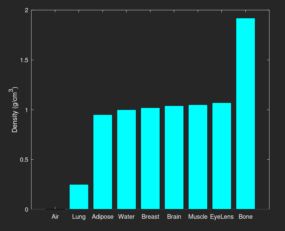
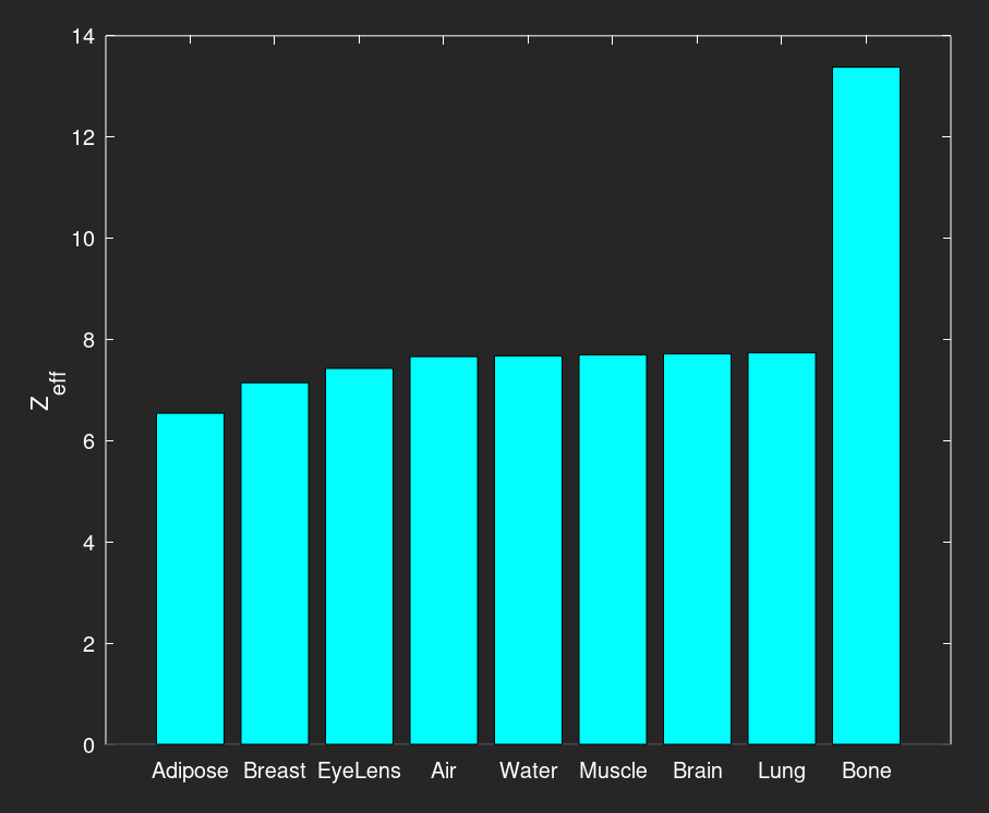
| Material | Density (g/cm3) | Zeff |
| Air | 0.001205 | 7.66 |
| Water | 1.0 | 7.67 |
| Adipose | 0.95 | 6.55 |
| Bone | 1.92 | 13.38 |
| Brain | 1.04 | 7.72 |
| Breast | 1.02 | 7.15 |
| Eye Lens | 1.07 | 7.43 |
| Lung | 0.25 | 7.74 |
| Muscle | 1.05 | 7.70 |
The effective atomic number Zeff was calculated using the power law method with an exponent of 3. In this study, we adjusted the physical density of lung to 0.25 g/cm3 to match what we see on clinical CT images, which is an air-lung mixture.
Source Code
The C++ code implementing the above methods can be found in the SolutioLabs project on Github. The ct_hu.cpp C++ file uses the SolutioCpp library, and ct_hu.m is the Octave code to plot the results.
Results & Discussion
Below is a bar graph of the various material densities, in increasing order. The majority of these materials are near 1.0 g/cm3 (water), except for air, lung, and bone.
This next figure is a bar graph of the various material effective atomic numbers, in increasing order. Notice the different material order when compared to the density graph.
The final figure is a bar graph of the HU values for each material, also in increasing order. Notice that while the material order is mostly the same as the density graph, breast tissue and water have switched places in the order. While breast tissue is more dense, it has a lower effective atomic number than water. This shows that the effective atomic number also has an effect on the CT number, and not just the density.
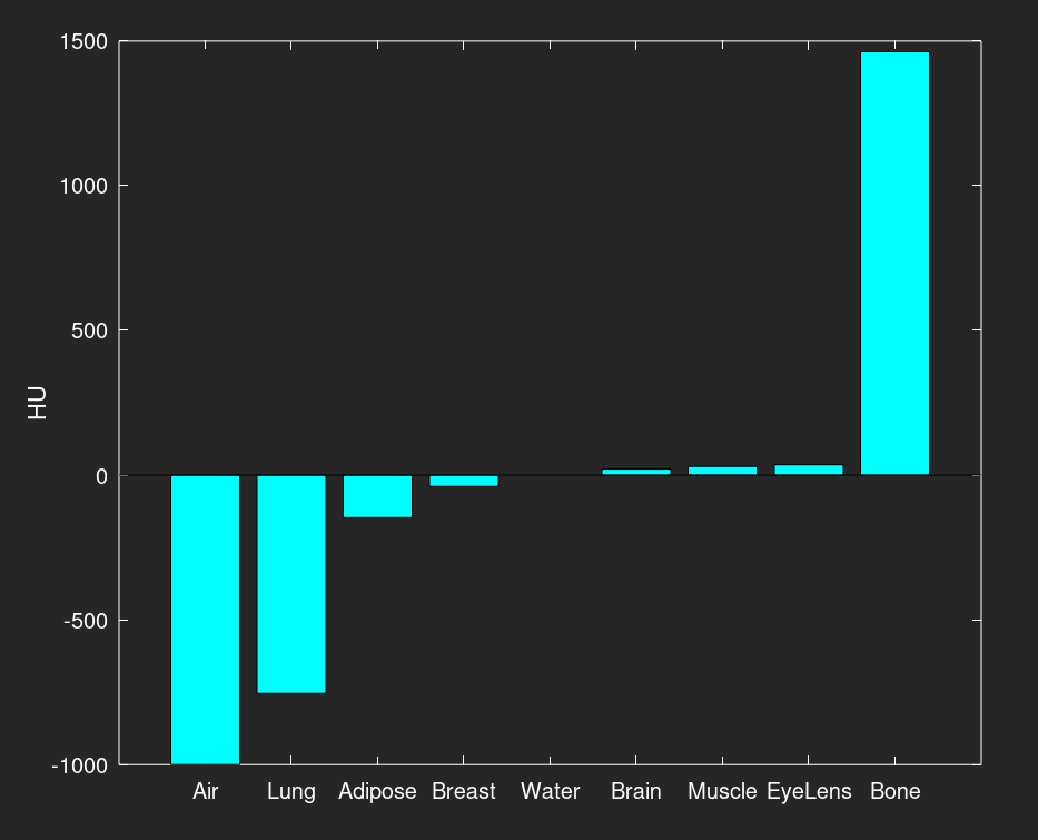
For a quantitative analysis, a table of the calculated HU values is shown below, along with sample values from the literature:
| Material | Calculated HU | Literature HU |
| Air | -1000 | -1000 |
| Water | 0 | 0 |
| Adipose | -147 | -150 to -50 |
| Bone | 1463 | 1000 to 3000 |
| Brain | 21 | 20 to 45 |
| Lung | -754 | -800 to -600 |
| Muscle | 30 | 20 to 50 |
The HU values for different tissues vary widely in the literature, so these table values are only approximate. Also, since the HU values for breast and eye lens tissue were not widely published, they were omitted from this table. Nonetheless, the calculated values agree well with the literature values.
Conclusion
It is possible to reasonably estimate the HU values for different materials in CT images, using NIST attenuation coefficients and TASMP x-ray energy spectra. The HU values for tissue depend on both the density and the effective atomic number of the tissue.